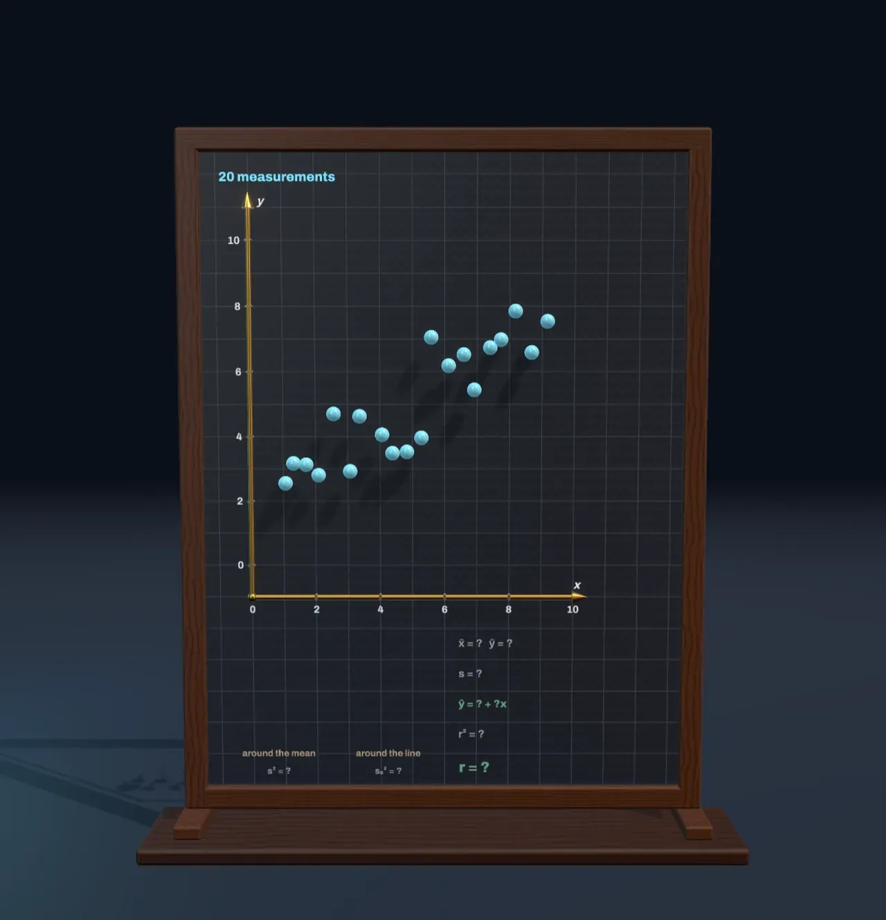
A cloud of measurements
Measure two things about the same objects and plot one against the other: the height and arm span of twenty people, the temperature and the ice-cream sales of twenty days, the weight hung on a spring and how far it stretches. Each object becomes one point, (x, y), and together they make a scatter plot. If the points drift upward from left to right, larger x tends to come with larger y; if they drift down, with smaller y. But real measurements never sit exactly on a line. Something else always nudges each one a little: other causes, chance, the limits of the ruler.
The board makes such a cloud from a rule you control. Every point starts on the straight line y = 5 + slope × (x − 5) and is then pushed up or down by a random amount. Slope sets how steeply the rule climbs or falls; Noise sets the size of the random pushes, the standard deviation of the draws. With Noise at 0 every point lies on the rule. The question statistics asks runs the other way: given only the points, find the rule and say how much to trust it.
The middle and the spread
Start with the y values on their own. Their mean, ȳ, is their total divided by how many there are. Step Fit the line to Mean and spread and a level line lights up at ȳ. The mean is the balance point of the data: the distances of the points above it add up to exactly the distances of the points below, so if each point were a weight on a ruler, the ruler would balance there. The ring marks the balance point of the whole cloud, (x̄, ȳ).
How far do the points stray from the mean? Each one’s distance to the line, its deviation, now hangs from it as a chalk stick, with a square drawn on it. Deviations above and below cancel when added, so statistics squares them first. The average of the squares is the variance, s², and its square root is the standard deviation, s (in many textbooks σ):
s = √( Σ(y − ȳ)² / n )
So s is the side of the average square, which stands beside the plot. The shaded band from ȳ − s to ȳ + s holds most of the points. For values that follow the bell curve it holds about two in three, and the band twice as wide about 95 in a hundred.
The line that misses least
Now step to Best-fit line. The level line turns about the balance point, and every stick follows it, so each stick becomes a residual: how far the line misses that point, measured straight up or down. As the line tips towards the trend the squares shrink, and it stops where their total area is as small as it can be. That is the least-squares line, or regression line, written ŷ = a + bx: a straight line, the linear function of school algebra, with slope b and intercept a.
The chart beside the Scene shows why there is exactly one such line. For every line through the balance point it plots the squares’ total area against the line’s slope; the curve is a parabola, and the best line sits at its lowest point. Working out where that is gives
b = Σ(x − x̄)(y − ȳ) / Σ(x − x̄)² and a = ȳ − b·x̄,
so the regression line always passes through (x̄, ȳ). With the starting values the board prints ŷ = 1.90 + 0.62x, close to the hidden rule, whose slope is 0.6. It is not exactly the rule, because these twenty draws of noise happen to tilt the cloud a little. Measure twenty more and the line would come out slightly different; how much it wobbles, and how that shrinks as the sample grows, is the subject of models and uncertainty.
Why squares, and not the plain distances? Squares are never negative, they make one large miss count far more than several small ones, and they lead to a single best line with a formula for it. Adrien-Marie Legendre published the method in 1805 and Carl Friedrich Gauss in 1809, both to fit the orbits of planets and comets to imperfect observations.
The correlation coefficient r
The squares also measure how well the line fits. Before the line, the squares about the mean have an average area of s². After it, the residuals’ squares have a smaller average area, sₑ². The share of the area the line removes is called r²:
r² = 1 − sₑ² / s²
and its square root, signed like the slope, is the correlation coefficient r. It runs from −1 to +1. At +1 or −1 every point lies on a line and no squares are left; near 0 the best line is almost level and removes almost nothing. With the starting values r = 0.89, so the line removes 78% of the area. The same number comes straight from the data as
r = Σ(x − x̄)(y − ȳ) / √( Σ(x − x̄)² · Σ(y − ȳ)² ).
As rough rules, an r above 0.7 in size is called strong and one below 0.3 weak. Karl Pearson put the formula in this form in 1896, building on Francis Galton’s work on heredity; Galton also gave regression its name, after noticing that tall parents tend to have children who are tall, but less so, closer to the average.
Try it: slide Noise to 0 and every point falls on the line: r = 1. Now slide it up to 2. The slope of the best line hardly changes, but the squares grow and r drops to 0.63. Then set Slope to 0.2 and Noise to 0: a gentle line, yet r is 1 again. r measures how tightly the points hug a line, not how steep the line is.
Outliers, curves and causes
Turn Outlier on and one bad reading appears, far below the rest. Its residual is large, so its square is huge, and because least squares weighs every square equally, that single point drags the line towards itself: the slope drops from 0.62 to 0.47 and r from 0.89 to 0.69. A real analysis would look hard at such a point before trusting the line, since a slip of the pen or a broken sensor can outweigh nineteen good measurements.
r measures only straight-line patterns. Points on a perfect arch, such as the height of a thrown ball sampled evenly from throw to catch, have r near 0 even though y depends on x exactly. Always look at the scatter plot, not just the number.
And a strong correlation does not say which way the cause runs, or whether there is one. Ice-cream sales and drownings rise and fall together, because hot weather drives both. Deciding what a correlation is evidence of needs more than the data on one plot; how evidence should shift a belief is the subject of Bayesian reasoning.
What this model leaves out
The noise is one fixed set of twenty random draws from a bell curve, rescaled so that their mean is exactly 0 and their standard deviation exactly 1, which makes Noise exactly the points’ spread about the rule. Their other properties are left as chance made them, which is why the fitted line is close to the rule but not on it. Only the y values are noisy: every x is taken as measured perfectly. Real data often have errors in both. And the method is lopsided either way: predicting x from y gives a different line from predicting y from x, unless r is ±1.
The spread s divides by n, as school statistics does. Many statistics books divide by n − 1 when the data are a sample from a larger population, which makes s a little larger. Every square is drawn on the plot’s own scale, so areas compare fairly, and each square is drawn on the side of its stick nearer the middle, only to keep it on the board.