One drop is not enough
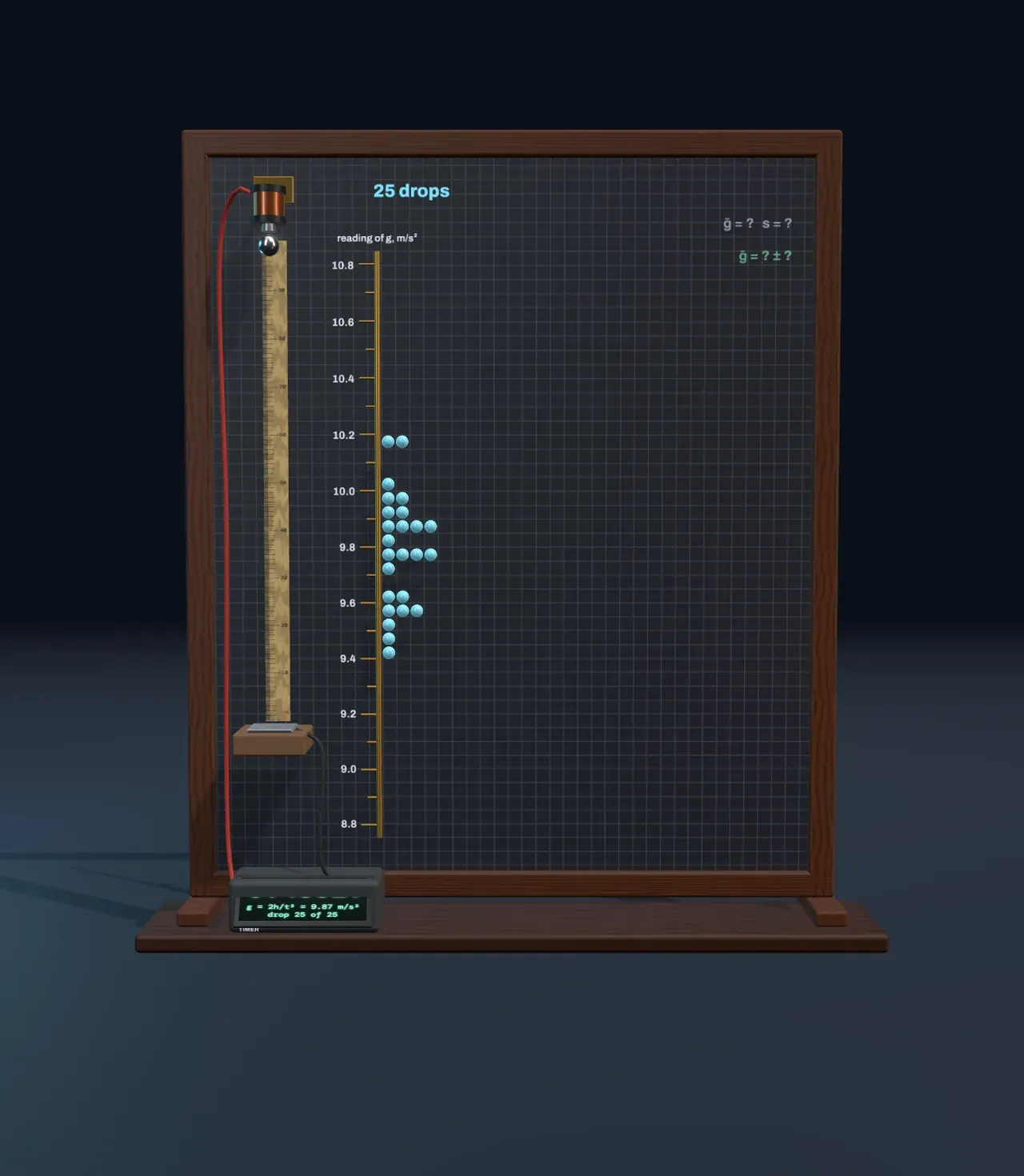
Hang a steel ball from an electromagnet, cut the current and time how long the ball takes to fall one metre onto a pad. The clock starts when the current stops and stops when the ball lands, and the time gives the acceleration of free fall through the rule for anything falling freely from rest, h = ½gt², or g = 2h/t². A fall of exactly one metre takes 0.4515 s if g is 9.81 m/s².
Now do it again. The second drop does not give the same time, and neither does the third. The ball twists a little as the magnet lets go, the contact on the pad closes a fraction early or late, and the readings land a few hundredths of a metre per second squared apart. The board on the right of the Scene keeps a tally: every drop becomes a ball on a pin, in the row of its reading, so the readings pile up along a scale from 8.8 to 10.8 m/s². The tally is a histogram lying on its side.
No single ball says how far off it is. The first drop on the board reads 9.63 m/s², which could be right to within a few hundredths or wrong by two tenths; nothing in one reading tells you which. Uncertainty is not a mistake to be ashamed of. It is part of every measurement, and the work is to say how big it is.
Random error and the spread
Errors that change from drop to drop, sometimes up and sometimes down, are random errors. Timing jitter sets their size: the standard deviation of the timing error, in milliseconds. Step Work out the true value to Spread and the board fits a model to the pile, a bell curve whose centre is the readings’ mean, ḡ, and whose width is their spread or standard deviation, s:
s = √( Σ(g − ḡ)² / (n − 1) )
With 25 drops and the starting jitter, the board prints ḡ = 9.79 m/s² and s = 0.20 m/s². The shaded band from ḡ − s to ḡ + s holds about two readings in three, as it does for anything that follows a bell curve. This is a model in the plainest sense: a short description, two numbers, that stands in for a pile of data and predicts where the next reading will probably land.
The spread describes one reading. Add more drops and the curve fills out, but it does not get narrower: the 100-drop pile is about as wide as the 25-drop one, s = 0.18 m/s². More drops do not make the timer steadier. Only a better timer does: slide Timing jitter down to 2 ms and the pile halves in width.
Try it: slide Drops from 1 up through 4 and 25 to 100. The pile grows into a bell, but its width stays about the same. Then try Timing jitter at 8 ms and at 2 ms.
Why the mean is surer: √n
What the experiment wants is not one reading but g, and the best estimate of g is the mean. The mean is far steadier than any single reading, because the random errors in it partly cancel: some drops read high, some low, and the more of them there are, the more closely the highs and lows balance. Step to Error bar. The bright vertical bar beside the pile is the standard error of the mean,
s/√n,
drawn as ± one standard error, with thinner whiskers out to two. With 25 drops it is ± 0.04 m/s², five times smaller than s, because √25 = 5. The result is written g = 9.79 ± 0.04 m/s².
The amber ticks beside the bar show what that number means. Each is the mean of another run of the same number of drops, 24 more runs that could have happened instead of this one. With 1 drop the ticks scatter as widely as single readings do. With 100 drops they huddle within a tenth of that, almost all inside the bar’s whiskers: the standard error is how far the mean of a repeat run would typically land from this one.
Because of the square root, accuracy gets expensive. To halve the error bar takes four times the drops, and to cut it by ten takes a hundred times. The chart beside the Scene plots s/√n against the number of drops: it falls steeply at first and then flattens, so the last drops buy little.
Systematic error
Now step to True value. A rose line marks the accepted value of g, 9.81 m/s², which a real experimenter would not know in advance. With 25 drops it lies inside the error bar: the gap is 0.6 error bars, as small as chance alone would often make it. Slide Drops up to 100. The bar shrinks to ± 0.02 m/s², the mean moves to 9.75 m/s², and the true value is now 3.5 error bars away. That is far more than chance explains.
The reason is the Magnet delay. Residual magnetism holds the ball for an instant after the current is cut, here 1.5 ms, so every timed fall is 1.5 ms too long and every reading of g about 0.065 m/s² too small. An error that pushes every reading the same way is a systematic error. Averaging cannot touch it, because it does not cancel: the mean of a hundred readings that are all 0.065 too low is 0.065 too low. The chart shows it at True value as a flat amber line beside the falling curve. Past the number of drops where the curve dips below it, about ten here, the systematic error is the larger, and more drops only make the wrong answer look more certain.
This is the difference between precision and accuracy. Random error spoils precision, how close the readings are to one another, and more data cures it. Systematic error spoils accuracy, how close they are to the truth, and more data does not help. A tight pile can be precisely wrong. A loose one can hide its bias: with 8 ms of jitter even 100 drops leave the 1.5 ms delay inside the whiskers.
Try it: set Magnet delay to 0 ms and Work out the true value to True value. Now every number of drops from two up agrees with 9.81. Slide it up to 5 ms: the whole pile slides down by 0.21 m/s², and the bar misses the line by more the more drops you take.
Finding a systematic error takes a different experiment, not a longer one. Change the method: drop from several heights and plot the square root of each height against its time. Since √h = √(g/2)·(t − delay), the points fall on a straight line that crosses the time axis not at zero but at the delay, and its slope gives g free of it (fitting such a line is the subject of statistics and regression). Or calibrate: time something whose answer you know. Checking results against independent methods is a large part of what the scientific method asks of an experiment.
Every result is a model
Writing g = 9.75 ± 0.02 m/s² is already a model of the measurement: each reading is the true value, plus a fixed systematic shift, plus a random error drawn from a bell curve. The ± says how wide the random part leaves the answer; it says nothing about the shift. That is why careful results list the two kinds of uncertainty separately, and why a disagreement between two careful measurements, each with a small error bar, is a clue that one of them has a systematic error nobody has found yet.
The physics is a model too. g = 2h/t² assumes no air drag, a point-sized ball and a clock that starts exactly when the fall does. Each of those is a small systematic error of its own. The statistician George Box put it in a line often quoted: all models are wrong, but some are useful. A good model is one whose errors are smaller than the uncertainty you need, and part of every measurement is checking that they are.
What this model leaves out
The readings are made from one fixed set of a hundred random draws, so the pile and its numbers are the same every visit; real repeats would differ. The random errors are bell-shaped and independent from drop to drop, which real timing errors only approximate: a pad that wears or a magnet that warms up would drift instead. The ball on the board falls in the time its reading took, as if there were no air. The spread divides by n − 1, as is usual for a sample, and the 24 repeat runs use their own fixed draws. The two-error-bar test is a rule of thumb: about one honest result in twenty lands that far from the truth by chance.