One trip, three questions
Roll a cart along a track and you can ask three things about it at every moment. Where is it? How fast is it going, and which way? Is it speeding up or slowing down? Each question has its own graph, drawn against time: position, velocity and acceleration.
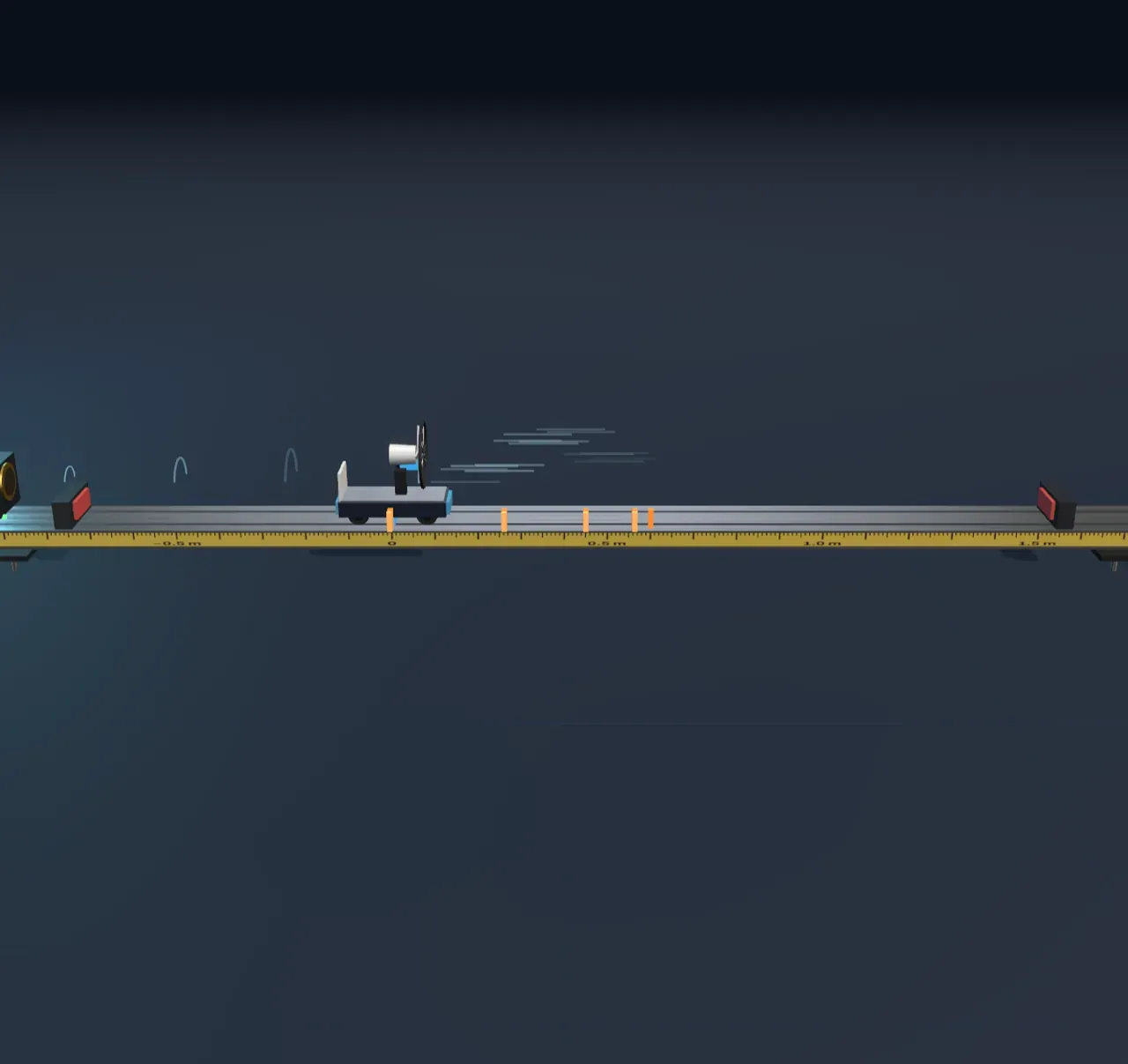
In the scene, a cart crosses the start line at the speed you choose, and a fan on its deck keeps pushing it with a steady force, forward or back. A motion sensor at the near end of the track times ultrasound echoes off the back of the cart, many times a second, and turns them into its distance. That is how school labs draw these graphs, and the chart beside the scene draws the cart’s position as the run happens. Orange marks drop on the track every half second, like a photograph taken with a flashing light: where they spread apart the cart is moving fast, and where they bunch up it is slow.
Try it: set Starting velocity to 0.6 m/s and Acceleration to −0.3 m/s². The cart sets off away from the sensor, slows, stops for an instant two seconds in, and rolls back to the start line just as the four seconds run out. The position graph is an arch.
Position against time
On a position–time graph, height is where the cart is, measured from the start line, and the horizontal axis is time. A cart standing still draws a flat line. A cart moving at a steady velocity covers the same distance every second, so its position rises (or falls) by the same step every second: a straight, sloping line. The steeper the line, the faster the cart.
A cart that is speeding up covers more distance each second than the last, so its line curves ever steeper. A cart that is slowing down curves the other way, levelling off. Where the curve reaches its top and turns over, the cart has stopped for an instant and started back.
The graph is not a picture of the path. The track is straight and the cart only ever moves along it, yet the graph curves. The curve is the story of the cart’s position through time.
Try it: set Starting velocity and Acceleration both to 0. The cart stays on the start line and the graph is flat. Then try a Starting velocity of 0.6 m/s with no acceleration: a straight line, rising 0.6 metres each second.
Velocity is the slope
How fast the position changes is the velocity. On the position graph, that is the slope: how much the line rises for each second along. Velocity has a sign. Positive means the cart is moving away from the sensor, negative means it is coming back. Speed is the size of the velocity, without the sign.
A curved position graph has a different slope at every moment. The slope at one instant is the slope of the tangent, the straight line that just touches the curve there. At the top of the arch the tangent is flat: the slope is zero, and so is the velocity.
Try it: step Build the graphs to All three graphs. The velocity and acceleration graphs fill in under the position graph, on the same time axis. A dashed tangent rides along the position curve, and its slope is the value the velocity graph is drawing at that moment.
Acceleration is the slope of velocity
How fast the velocity changes is the acceleration, and it is the slope of the velocity graph. The fan’s steady push gives the cart a constant acceleration, so the velocity graph is a straight line and the acceleration graph is a flat one.
A negative acceleration does not always mean slowing down. With the cart rolling forward at 0.6 m/s and the fan pushing back, the acceleration is −0.3 m/s² the whole time. For the first two seconds the velocity is positive and shrinking, so the cart slows. After it turns round, the velocity is negative and growing in size, so the cart speeds up, backwards. The cart slows down when its velocity and acceleration have opposite signs, and speeds up when they share one.
The area under the velocity graph
If a cart moves at 0.5 m/s for 2 seconds, it travels 1 metre. On the velocity graph that motion is a rectangle 0.5 high and 2 wide, and its area, 0.5 × 2, is the 1 metre. The same holds for any shape: the area between the velocity graph and the time axis is the change in position, the displacement.
Area above the axis counts as forward and area below counts as backward. Over the default run, the triangle above the axis (the trip out) and the triangle below it (the trip back) have the same size, so they cancel: after four seconds the cart is back where it started, with a displacement of zero, although it has travelled 1.2 metres. That total, counting both ways, is the distance travelled.
Try it: step Build the graphs to Area under velocity. The area fills in as the cart moves, its sum is printed under the graphs, and an arrow on the track spans the same displacement from the start line.
The equations of constant acceleration
For a cart that starts with velocity u and has a constant acceleration a, the graphs give three equations. The velocity graph is a straight line starting at u with slope a:
The area under it, a rectangle u × t plus a triangle ½ × t × at, is the displacement:
Taking t out of the two gives a third, handy when the time is not known:
With u = 0.6 m/s and a = −0.3 m/s², the first says the cart stops when t = 2 s, and the second puts it 0.6 m from the start line at that moment. The third gives the same 0.6 m without the time: 0 = 0.36 − 0.6x.
What the model leaves out
A real fan cart’s push wavers as the motor warms up and the battery runs down, and the wheels and air slow it a little, so a real velocity graph is never perfectly straight. The scene keeps the push exactly steady and leaves friction and drag out. The cart crosses the start line already moving; the push that set it going is not shown.
The scene computes the cart’s position from the equations rather than measuring it, so its graphs are smooth. A real motion sensor reads the position a few dozen times a second, each reading slightly off, and software works out the velocity and acceleration from the differences between readings, which makes them noisy, the acceleration most of all. The end stops halt the cart and end the run at once, without the bounce a real bumper would give.